
Grouped and Ungrouped data is very common in statistics. Data items can be considered as a group. This approach works well when the number of records is huge. It is more efficient than considering an individual item.
Grouped Data
Grouped data, on the other hand, is a way of organizing data into intervals or classes. These intervals represent a range of values, and data points are grouped within these ranges. This method is used when dealing with large datasets, where it’s not practical to work with individual data points. The table below illustrates grouped and ungrouped data.
Key Characteristics of grouped data includes:
- Organized into classes/intervals: Data is organized into ranges or categories.
- Simplified analysis for large datasets: Helps to summarize and analyze large sets of data.
- Class intervals: These represent a range of values within which the data points fall.
- Frequency distribution: A frequency table often accompanies grouped data, showing how many data points fall into each interval.
Ungrouped and ungrouped data question
we will be discussion various problems involving grouped and ungrouped data. Ungrouped data is also known as raw data or unorganized data. It refers to individual data points that are not organized into categories or intervals. Each value is listed separately, and there is no summarization or categorization.
Key Characteristics of ungrouped data includes:
- Raw format: The data is presented as a simple list of individual values.
- No grouping or categorization: Data points are not grouped into ranges or classes.
- Easier to analyze for small datasets: Suitable for small datasets, where you can analyze each value individually.
In grouping, you take few neighboring items and put them in a group. For example, if you have items like 41,42,42,43,45,46, you can decide to consider a group of 41-45. This approach avoids listing the numbers individually.
Let us consider the data provided below that shows ages of some 20 senior workers in a company:
63, 53, 58, 64, 54, 64, 58, 67, 54, 54, 56, 53, 51, 52, 58, 53, 63, 65, 67, 58.
we can make the frequency table as we discussed earlier
| Age | Tally | Frequency |
| 51 | / | 1 |
| 52 | / | 1 |
| 53 | //// | 4 |
| 54 | // | 2 |
| 56 | / | 1 |
| 58 | //// | 4 |
| 63 | // | 2 |
| 64 | // | 2 |
| 65 | / | 1 |
| 67 | // | 2 |
| Total | summation | 20 |
ungrouped data of senior workers in a company
63, 53, 58, 64, 54, 64, 58, 67, 54, 54, 56, 53, 51, 52, 58, 53, 63, 65, 67, 58.
We can reduce the size of the table by grouping the data in 5 values as shown. Please note that we have changed the first column from age to class. This means it will represent a class of a certain age group.
| class | Tally | Frequency |
| 51-55 | 8 | |
| 56-60 | 5 | |
| 61-65 | 5 | |
| 66-70 | // | 2 |
| Total | summation | 20 |
Grouped data for senior workers in a company
Measurements like height, mass, age, time etc. are usually estimates of the actual values so any value between 50.5 and 51.4 is estimated as 51. Thus we can write interval x as 50.5 ≤x< 51.5.
A class interval 51-55 includes all masses between 50.5 t0 55.5
The values 50.5 and 55.5 are called the class boundaries of the class 51-55.
50.5 is the lower class boundary in this case and 55.5 is the upper class boundary.
The difference between the class boundaries is the class width(class size). For example in the example above, class width =55.5-50.5 = 5
when grouping data, ensure the groups are not so many, the most recommended is 5-12 groups.
practice question : Grouped and ungrouped data
The data below shows masses of 30 animals in animal farm.
27, 28, 24, 25, 30, 40, 30, 28, 26,43, 27, 28, 33, 35, 36,
27, 30, 28, 31, 30, 28, 29, 30, 35, 32, 26, 25, 42, 43, 27.
Required:
(a) Make a grouped frequency table for the data
(b) represent the grouped data in a bar graph and then in a pie chart4
Solution
The first step is deterring the number of classes. This we do by determining the range and the size of each group. let say each group should have n items and the range is R.
The number of groups (classes=R/n) approximated to the nearest whole number that is greater than R/n.
the range is the difference between the highest score and the lowest score. In the above data, the range = 43-24 = 19
Assuming we want each class has five items, then number of classes = 19/5≈3.8 which should be 4 to the nearest whole number. however we said the best numbers is between 5-12. hence we can reduce the number of items per group, to 4.
hence 19/4 = 4.75 classes ≈5
Five classes are better than four. This is because a fewer number of items in a group can increase accuracy. This increase is noted when calculating the measures of central tendencies.
the groups starts from the lowest value, and then add 3 items to get the upper boundary of that group. Note we have added 3 and not 4. The lower boundary needs 3 more items to make 4 items in the group.
The frequency table for the grouped data should be as follow
| classes | Tally | Frequency |
| 24-27 | 9 | |
| 28-31 | 12 | |
| 32-35 | //// | 4 |
| 36-39 | / | 1 |
| 40-43 | //// | 4 |
| Total | summation | 30 |
Frequency table for masses of animals in a farm
The data can be represented in the in a bar graph as shown

Practice question
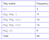
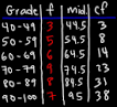
The marks obtained by students in a Java test were recorded as follow
71, 73, 64, 58, 49, 52, 62, 68, 52, 48, 55, 63, 60, 71,
66, 61, 58, 57, 65, 64, 49, 52, 59, 53, 59, 74, 56, 57, 59,66.
required:
- make a frequency distribution table for the data
- Draw a histogram to show this information
Related Topics
- Introduction to statistics
- Bar Graphs: concise Introduction1
- Measures of dispersion
- Grouped and ungrouped data
- bar graphs
- Line graphs
- Frequency polygon
- Histograms
- pie charts
- Measures of Central tendency
Leave a Reply