Quartiles divides a set of data into four equal parts.
A median divides a set of data into two parts each with equal number of items.
The first quartile, mostly referred to as the lower quartile contains 25% of the total data items. Lower quartile can be described as the median of the bottom half.
Second quartile is actually the median of the whole data(50%).
The third quartile is usually referred to as upper quartile and contains 75% of total data items. It can be described as the median of the upper half the data set.
Formula for the getting the first quartile Q1

Where
- L is the lower class boundary of the quartile class.
- n is the total frequency
- c is the cumulative frequency above the quartile class
- i is the class interval
- f is the frequency of the lower quartile class
Formula for the getting the second quartile Q2
Second quartile Q2 is actually the median of the data
it is calculated from:

where
- L is the lower class boundary of the median class.
- n is the total frequency
- c is the cumulative frequency above the median class
- i is the class interval
- f is the frequency of the median class
Formula for the getting the third quartile Q3

where
- L is the lower class boundary of the upper quartile class.
- n is the total frequency
- c is the cumulative frequency above the third quartile class
- i is the class interval of the upper quartile class
- f is the frequency of the upper quartile class
Deciles
Deciles divides a set of data into ten equal parts.
First decile is when n is divided by 10. that is; Decile = n/10
where n is the total frequency for the data
Percentiles
Percentiles divides a set of data into hundred equal parts.
one percentile is given as (1/100)*n
In quartiles, deciles and percentiles, data is arranged in ascending order
Example 5
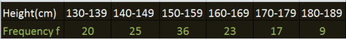
The table below shows the distribution of heights to the nearest cm of students in a school.
Find (a) the median
(b)(i) lower quartile (ii) upper quartile (iii) 80th percentile.
Solution
(a) The new frequency table for the data is shown here
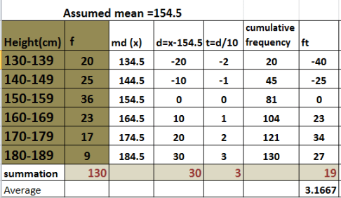
There are 130 students . Therefore, the median height is the 65th student. that is; median is 130/2.
The 65th student falls in the 150-159 class. This class is called the median class.
Using the formula for the median:

(b) (i)
Lower quartile Q1 = L + (n/4 – C)i/f, that is:

ii)
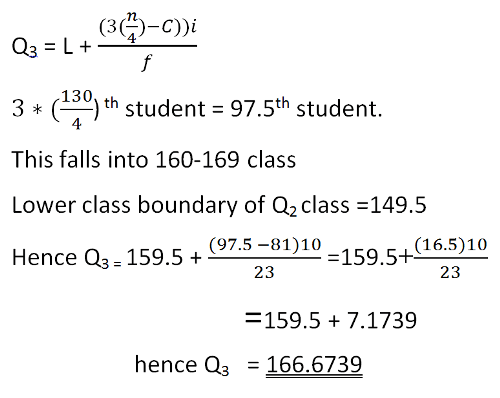
Upper quartile Q3= L + (3n/4)-23)*5/9
(C)
The 80th percentile of the data is given by 80/100)*130=104th value.
The 104th student falls in the 160-169 class
80th percentile= L+(80/100n-C)i/f
The complete solution is as below:

Example
Determine the lower quartile and upper quartile for the following set of data
15, 20, 16, 15, 18, 17, 13, 9, 17, 18, 11
solution
arranging in ascending order
9, 11, 13, 15, 15, 16, 17, 17, 18, 18, 20
The median number is 16. On left of 16 there are 5 values and on the right 5 values.
16 is at the center of the data list
9, 11, 13, 15, 15 | 16 | 17, 17, 18, 18, 20
The first half contains: 9, 11, 13, 15, 15
The central value in that lower half is 13 and it is the first quartile of the data
The upper half includes: 17, 17, 18, 18, 20
The central value is 18 and is hence the upper quartile for the data list