comprehensive study approach

Tag: F

Characteristics of Wave Motion
The characteristics of a wave motion can be explained with reference to the oscillatory motion of mass attached to a spring or by use of a bob on a swinging pendulum.

The figure below shows a mass that is attached to a spring and one end and fixed on the other end as shown

illustrating mass oscillating on a spring

Initially, the mass is at rest at the end of the spiral spring at position M. The mass is then depressed slightly to position L and released and is then observed that it oscillates up and down about the mean position M.

One complete oscillation occurs when the mass moves through positions N-M-L-M-N. That is, it makes one complete oscillation when it has returned to it’s starting position and is moving in the same direction. For example if the mass starts at M the move to M-N-M, it will not have moved a complete oscillation because although it has returned to it’s starting position, it is moving in the opposite direction.

Consider a swing pendulum shown below

illustrating swinging pendulum

For the pendulum, the bob makes a complete oscillation when after an initial displacement from position X, the pendulum swings through position X-Y-Z-Y-X. If the mass in the above diagram takes two seconds to make a complete oscillation, a sketch of it’s time-displacement graph for the motion will be as shown below.

Displacement time graph for a swinging pendulum

As can be seen from the above diagram, the displacement time graph for an oscillatory motion is a sine curve similar to the transverse wave profile.

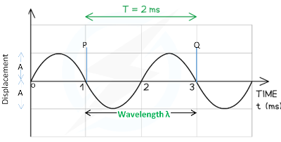
To describe the general characteristics of a wave motion, consider the motion-time graph representing a certain wave motion as shown below

To illustrate wave characteristics

The Displacement value A shows the maximum displacement A from the mean position o.

P and Q are said to be points in phase because the wave pattern is repeating itself at Q and P.

The distance between two points in phase is called the wavelength λ. The distance between P and Q represents on wavelength.

The wave starts repeating itself at P before repeating itself again at Q. Hence when the wave moves from P to Q, it is said to make one complete oscillation.

The time taken to complete one oscillation is known as the Periodic time T. In the motion-time graph above, the periodic time is two milliseconds(ms) as it has taken 2ms to make one complete oscillation.

Two points in a wave are said to be in phase, if they are in the same position, relative to the wave profile. P and Q are in phase.

The number of oscillations that can be made by a wave motion in one second is called the frequency f of the wave and is usually the reciprocal of the periodic time.

from the above diagram, it takes 2ms to make one complete revolution which is equivalent to (2/1000)s = 0.002 Seconds.

The frequency of the wave can then be determined as follow:

It can be shown that:

Where T is the periodic time and f the frequency of a given wave

Related Topics
February 20, 2024
Working with assumed mean
Assumed mean is a certain value that is chosen from the data set such that it can be subtracted from all other values to reduce the size of numbers in the data set.

An assumed mean is usually determined by guessing the number that could be used as the mean among the values in the data set.

It is like picking one of the numbers in the dataset and assuming it is the mean for the data. By looking at the data, we can guess a number close to the mean because mean, as a measure of central tendency, which most likely will be a number near the median of the data.

Take for instance the data set below.

89, 64, 56, 78, 88, 67, 72, 85, 70, 65, 64, 66, 72, 74, 76.

Arranging the data in ascending order we have

56, 64, 64, 65, 66, 67, 70, 72, 72, 74, 76, 78, 85, 88, 89.

Range= 89 – 56 =33

A method I find convenient to find a central data item is 56+(33/2) =56+17=73.

Now because we don’t have 73, I pick 72 as the assumed mean. And I will subtract 72 from each data item as in table below.

Now i get the summation of fd: ∑fd=-1

and mean of d= (∑fd)/(∑f) ≈ -0.06667

mean of x, x̄ = 72 + (-0.0667) = 71.9333

The sum of x has been done by a statistical software. Otherwise it could be time consuming and error prone and energy sucking to try and compute it manually. It has been recorded there for comparison purposes.

in a more general case, if we take an assumed mean A and subtract it from each data item x, then we get data items labelled with d such that d=x-A and the mean for the data expressed as:

Practice question

Using an assumed mean, calculate the mean of each of the following sets of data

(a)

0.655, 0.685, 0.705, 0.665, 0.695, 0.715, 0.375, 0.745, 0.755, 0.765, 0.745, 0.550, 0.450, 0.400, 0.425, 0.325, 0.775, 0.685, 0.695, 0.745

(b)

225, 400, 300, 225, , 525, 325, 600, 225, 325, 400, 525, 575, 625, 250, 650, 350, 475, 550, 575, 275, 375, 475, 475, 675, 400, 375, 275, 250.

Related Topics
January 30, 2024
Vocabulary used in Thin Lenses
In summary

Thin lenses have their own vocabulary mostly that describes various parts of the lens. This parts includes:
- Center of curvature C
- Radius of curvature R
- Principal axis P
- optical center O
- Principle Focus F
- Focal Length f
- Focal plane
We will discuss all the highlighted parts in this lesson

Center of Curvature C

It is defined as the center of the sphere of which the surface of the lens is part.

We consider the lens to have been cut off from a transparent sphere of radius R. In other word, the lens is part of a curved surface of a certain sphere as illustrated below.

For bi-convex lens, the lens is considered to come from two pieces cut from two different spheres and combined at the inner side. Consider the illustration below where we extract service1 and service2 from two spheres.

sphere for surface1

sphere for surface2

Because the bi-convex comes from two spheres, it will have two centers of curvature which will be opposite to each other.

similarly the bi-concave lens is derived from two spheres as illustrated.

Different parts from spheres will be joined two have a concave lens that has two centers of curvature as shown below

Radius of curvature

It can be defined as the radius of the sphere from which the surface of the lens is part.

It can also be defined as the distance between the Center of curvature and the optical center o of the lens.

Principal axis

It is an imaginary line passing through the centers of curvature and is perpendicular to the plane of the lens.

Optical center

It is the geometric center of the lenses where a ray incident to the lens passes on undeviated.

Principal focus

Sometimes also referred to as the focal point. It is a point on the principal axis where rays parallel and close to the principal axis converge after refraction by a convex lens or where the rays parallel and close to the principal axis seems to diverge from after refraction by a concave lens.

The figure below illustrates convergence of parallel rays of light at principal focus after refraction.

showing a principal focus of a convex lens

The virtual principal focus of a concave lens is as illustrated below

A lens has two principal foci, and they are on either side of the lens.

The principal focus of converging lens is said to be real because their actual meeting of rays of light there.

The principal axis of diverging lens is said to be virtual (imaginary) because rays of light do not actually meet there.

Rays that are parallel and close to the principal axis or almost parallel to the principal axis are referred to us paraxial rays.

Rays parallel but far from the principal axis are referred to as marginal rays or axial rays.

Focal length f

It is the distance between the optical center of the lens and it’s principal focus.

By Convection, focal length of converging lens is considered real while that of diverging is considered virtual.

Focal plane

It is an imaginary plane that passes through the focal point and is perpendicular to the principal axis.

Focal plane is illustrated below

rays of light that are not parallel to the principal axis converges at a point on a focal plane or will appear to diverge from there after refraction

Conclusion

In this lesson we have seen that lens are pictured as being extracted from a sphere and the radius of the said sphere plays and important role in description of the lens. A lens converge or diverges rays parallel to the principal axis at the focal point.

Related Topics
- Thin lenses
- Physics
References
- IGCSE Physics, third edition(Tom Duncan & Heather Kennet, 2014)
- High school physics(OpenStax University, 2020)
January 14, 2024