Sometimes measures of central tendency does not give the actual picture of the data in question. For example if we were to determine the average income per home of a certain country, we may obtain a high value and fail to deduce that majority of people have been living below poverty line but are dominated by few individuals that earns extremely high incomes. The few people earning very high income raises the average earning and the mean may wrongly be interpreted by assuming that the people living in such a country are wealth people.
Dispersion can be used to measure how values are spread from the minimum value to the maximum value.
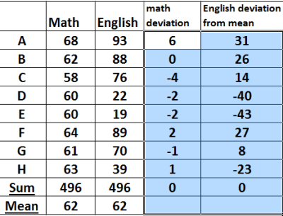
Consider the table below

The table shows scores of some students in a Math and English test.
But a mean may fail to show that one class has extreme case of a bright student and of a not so bright one. The first data shows that all the students in class are of average ability.
The data in math has a small range of 68-58=10 but English has a wide range of 93-19=74. Yet the two subjects have the same mean as their totals are the same but Marks in B are more spread out than in A.
One measure of dispersion is the range which represents the difference between the highest and lowest value in the data set. However, a range may have limitations because it uses two extreme values that may have strayed from the true picture of actual observations.
A county may have lower value for income per home but the quality of life is high because there are not cases of extreme poverty and the gap between rich and poor is not that wide like what happens in Africa.
Inter-quartile range
It is the difference between the lower and the upper quartile and consists of the 50% of the whole data that is usually close to the mean and other measures of central tendency.
Semi inter-quartile range
It is also called the quartile deviation and it represents the average between upper quartile and the lower quartile. It is usually obtained by adding lower quartile and upper quartile then dividing by two.
Mean deviation
Mean deviation is the difference between each value and the mean for the data. It is obtained by subtracting the mean from each value of the data set. The table below shows deviation from the mean of the math and English test shown above. please note that the sum of deviations from the mean is zero.
Mean absolute deviation
The sum of deviations from the mean sums up to 0. This is because mean is usually at the center of all values in the data set. Subtracting means from values left of the mean gives negatives deviation and those from right gives positive deviation. The table below shows that extract of columns of deviations from the mean of the previous data.
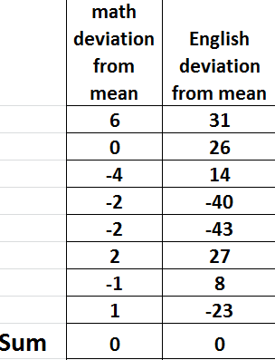
To have a meaningful insights from the deviations from the mean, the negative values are ignored so that only positive values are considered. Hence we talk about the absolute values from the mean.
The sum of the absolute deviations from the mean are summed up then divided by frequency to have the mean absolute deviation.
Consider deviations from the mean from the previous data we have discussed. Now we have ignored the the negative sign and included only the number alone without considering it’s sign as shown.

As can be seen from the table above, the mean value for math is only 2.25 whereas for English where the range is big, the mean is 26.5, which is much higher compared to math.
Variance
Instead of finding absolute values, we square each deviation so that each deviation results is made positive.
Variance is the sum of the squared deviations from the mean, divided by the frequency.
Related Topics
- Assumed mean
- Introduction to statistics
- Measures of dispersion
- Grouped and ungrouped data
- bar graphs
- Line graphs
- Frequency polygon
- Histograms
- pie charts
- Measures of Central tendency
- Mean for grouped data
- Working with the assumed mean
- Quartiles, Deciles and percentiles
- Measures of dispersion
- Variance