Cartesian plane is used as a frame of reference for points in a line. It has two lines that intersects at the center of a page such that they divide a grind page into 4 parts.
If you can remember the concept of number lines, Cartesian plane is made of two number lines, one horizontal and another vertical, where there zero point meets at the center of the page.
The points where this two lines meet is usually referred as the origin.The horizontal line in the Cartesian plane is refered to as the x-axis. The line drawn vertically is usually referred to as the y-axis.
For each axis, a suitable scale is chosen and then marked at equal intervals. The measurements on the axes are called the coordinates.
The coordinates are given as an ordered pair (x,y) with x-coordinate first and y-coordinate second.
The two coordinates are separated by a comma and are placed inside brackets.The planes on which the points lies is called the Cartesian plan .
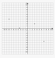
Example
Write down the coordinates of the following points:
Assumed mean is a certain value that is chosen from the data set such that it can be subtracted from all other values to reduce the size of numbers in the data set.
An assumed mean is usually determined by guessing the number that could be used as the mean among the values in the data set.
It is like picking one of the numbers in the dataset and assuming it is the mean for the data. By looking at the data, we can guess a number close to the mean because mean, as a measure of central tendency, which most likely will be a number near the median of the data.
A method I find convenient to find a central data item is 56+(33/2) =56+17=73.
Now because we don’t have 73, I pick 72 as the assumed mean. And I will subtract 72 from each data item as in table below.
Now i get the summation of fd: ∑fd=-1
and mean of d= (∑fd)/(∑f) ≈ -0.06667
mean of x, x̄ = 72 + (-0.0667) = 71.9333
The sum of x has been done by a statistical software. Otherwise it could be time consuming and error prone and energy sucking to try and compute it manually. It has been recorded there for comparison purposes.
in a more general case, if we take an assumed mean A and subtract it from each data item x, then we get data items labelled with d such that d=x-A and the mean for the data expressed as:
Practice question
Using an assumed mean, calculate the mean of each of the following sets of data
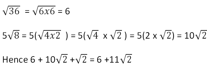
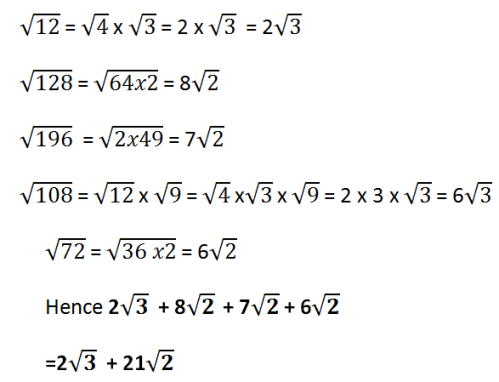
To simplify expressions involving surds, we simply add or subtract coefficient of irrational factors that are alike. thus
To simplify surds, you want to express them in their simplest form typically by factoring out any perfect square factors from the radicand (the number under the square root symbol).The steps to follow includes:
Identify the perfect square factors: Look for perfect square numbers that evenly divide into the number under the square root. For example, in √72, the perfect square factor is 36 because √36 equals 6.
Factor out the perfect square: Rewrite the surd using the perfect square factor outside the square root. For example, √72 becomes 6√2.
If possible, simplify further: Sometimes, you can simplify the expression even more. For instance, if you have √18, you can factor out √9 from it to get 3√2.
Repeat if necessary: If there are still perfect square factors remaining under the square root, repeat the process until you can no longer simplify.
Example
solution
(a)
(b)
The idea is to express 12 as products of two numbers. One number results to a rational number after the split. similarly, 128 can be expressed as a product of 64 and 2 such that square-root of 64 results to a rational number.
After expressing all the terms in a simplified for , then some of them will have same irrational factor and hence they can be added to make them simpler.
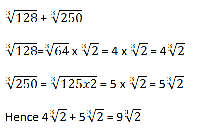
(c)
The idea is to express 128 into two factors such that it is possible to find the 3rd root of one of them and get a whole number. From quick inspection, 128 =64 x 2 and third-root of 64=4.
similarly we can express 250 as a product of 125 and 2. We can be able to deduce that 125 is cube of 5 and hence cube-root of 125 is a rational whole number.
The solution will involve changing the surds so that they can be of the same order. Then we can compare their values from inside the root.
Like and unlike surds
Surds are alike if they have the same irrational factor, otherwise they are unlike surds.
Example
Solution
27 and 12 can be simplified such that they become a product of both rational and irrational numbers.
like 27 is a product of 9 and 3. and when we get the squareroot of 9, we gat a rational number 3.
similarly, 12 is a product of 4 and 3 and when we write 4 under square-root, it results to 2 which is rational. now both 12 and 27 and 1/3 when simplified will have the same irrational number as shown below
To simplify expressions involving surds, we simply add or subtract coefficient of irrational factors that are alike. thus
In grouped data, there need a value that can be used in each group so that we can get ∑fx for each class and eventually summation of values to get the mean. The value used to represent values of a given class is the midpoint (x) obtained by adding lower and upper class boundary and dividing them by two.
Example
The frequency table below shows masses in kilograms of some grade 10 students.
class
Frequency
60-64
8
65-69
7
70-74
12
75-79
9
80-84
6
85-89
5
a table showing frequency against group of ages
Required:
(a) State the modal class
(b) Estimate the mean
(c) Estimate the median
solution
(a) The modal class is 70-74 because it has the highest frequency (12).
(b) we redraw the table to include a column for the midpoint values
the midpoint of class 60-64=(60+64)/2 = 62, and you will follow the same step to get midpoints of other classes which will include 67,72,77,82 and 87.
Mean x̄ = (∑fx)/(∑f)
hence Mean x̄ = (3449)/(47) = 574.833
(c) The median value is the value at the 24th position of the frequency. This is because of all the data were arranged in ascending order, the middle one would be at the 24th position. On the left of 24, there would be 23 values and on the right there would be 23 values.
if we add the frequencies cumulatively we have 8, 15, 27, 36, 42, 47 respectively. It means there are 27 values with 74 kg and below, the middle value (24th value) is found in the class 70-74.
The lower class boundary of the median class is 69.5 kg. which best fits the mass of the 15th person.
to get the mass of the 24th person ,we need 9 people from the median class.
so we get 69.5 + ((24-15)/12) * 5 = 69.5+3.75 = 73.25
Exercise
(a) The table below shows the masses of some people that visited a hospital
Class
Mid-point(x)
frequency f
fx
51-55
9
56-60
13
61-65
15
66-70
17
71-75
24
a table of masses of people that visited a hospital
(a) copy and complete the table
(b) Find:
The mean
The Median
(b) The height in centimeters of 25 people were measured as follows:
(a) Using a class width of 5 make a grouped frequency table
(b) from the table estimate:
The mean
The median
solution
(a) The lowest value is 156 and so the first group will be 156-160, the highest value is 190. The range is 190-156=34.
34/5=6.8 ≈ 7.
So there is about 7 groups. We develop a table as shown
(b) The formula for calculating the mean is
∑fx=4265 as read from the table
∑f = 25
hence
The total number of items, which is the summation of frequency (∑f) is 25.
The median, which is the number at the center is the 13th value
The class that will contain 13th value is a class that starts with 10th and ends with 14th value as shown in the table. That class is 166-170 and it is the median class.
The lower class boundary of the median class is 165.5
The cumulative frequency above the median class is 9
The frequency of the median class is 5
The formula for the median is given as
where L is the lower class boundary of the median class, n the total frequency, C the cumulative frequency below the median class, i the class width and f the frequency of the median class
Hence the median of the data is 169
(c) The average temperatures at a weather stations were recorded for 30 days as follow.
Mass is the quantity of matter in a substance. Matter is anything that occupies space.
The mass of an object depends on it’s size and the number of particles it contains.
The SI unit of mass is the Kilogram (Kg).
A kilogram is the mass of a piece of platinum-iridium metal kept at Sevres, near Paris,France at the International Office of Weights and measurements. That piece of metal kept in France is the standard with which all masses of the world are measured with the kilogram unit.
though kilogram is the SI unit, the most common unit of measuring mass is the gram.
The following table shows sub-units of gram and kilogram
Prefix
number of grams (g)
Kilogram (Kg)
1000 g
Hectogram (Hg)
100 g
Decagram (Dg)
10 g
decigram (dg)
(1/10) g
centigram (cg)
(1/100) g
milligram (mg)
(1/1000) g
microgram (µg)
(1/1000,000) g
nanogram (ng)
(1/100,000,000) g
picogram (pg)
(1/1000,000,000,000) g
tables of conversion of grams
1 kg = 1000 tonnes
other units used to measure mass includes:
1 pound (lb) = 0.4536 kg)
1 ounce(oz) = 0.02835kg
Though different weights are experienced depending on gravitational pull of a place, the mass of an object remains constant beacuse number of particles in an object will not change with change of location.
Instruments used to measure mass
Platform balance
Electronic balance
The object whose mass is to be measured is placed on the pan and its weight causes electronic circuit to develop current to display the mass on the digital display. It is a very accurate instrument and is useful in laboratories especially small masses.
Beam balance
works by the principles of moments.
The object whose mass is to be measured is balanced against a known standard mass on as equal arm lever. The beam balances when the mass of the object is equal to the standard mass.
Table balance
works under principles of moments
Spring balances
uses laws of gravitational pull
postal balance
Roman Steelyard Balance
Exercise
convert the following as instructed
1500 tonnes to kg
200000000000 mg into Kg.
256 g into tonnes
0.000000000000000000 567 tonne into pg
12.43 g into mg
Problems involving mass
Sheila went to the grocery store and bought a 3 watermelons that weighed 4.4 kilograms and a bunch of bananas that weighed 750 grams. She also bought a bottle of juice that contained 1.2 liters.
a) Convert the weight of the watermelon from kilograms to grams.
b) If Sarah bought 3 bottles of juice, how many grams of juice did she buy in total if density of juice is 1.25gcm-3?
c) If each banana weighs 125 grams, how many bananas did Sarah buy?
Measures of central tendency in statistics are single values that can be derived from the data set such that it can be used as the representative of the whole data.
The most common measures of central tendency includes:
Mean
mode
Median
Mean
Mean is the average value for the data set. It is obtained by finding the total sum of all the values in the data set then divining it by the total frequency.That is;
Mean = (Sum of all Values)/(Total frequency)
consider the following set of data represents marks scored by a group of students in a math test:
68,65,59,30,42,45,46,59,80,23,54, 45,54,30
The sum of values in the data= 68+65+59+30+42+45+46+59+80+23+54+45+54+30=700
The total frequency of the data set = 14 because there are 14 results in the test
Mean = 700/14 = 50
Mean value could be interpreted to mean the value that could result if data set was modified so that each item will have the same quantity.
Example Problem
10 athletes measured their masses which were recorded and their mean determined as 60.45 Kg. The mass for nine of them were 62.10kg, 58.90kg,56.8kg, 49.70kg, 57.1kg, 64.56kg,58.35kg,55.21kg, 58.67kg but the weight of one athlete was never recorded. Help determine the missing mass.
Solution
Mean = (Sum of all Values)/(Total frequency)
let the missing value be x
then total mass for the ten athletes will be 62.10+58.90+56.80+49.70+57.1+64.56+58.35+55.21+58.67+x
frequency = 10 as there are 10 athletes
but mean = 60.45
hence 60.45 =(521.39 + x)/10
hence 604.5 = 521.39+x
x=604.45 – 521.39 = 83.06 kg
Practice Question
Four numbers have the following number of animals: 134, 233, a, 2a. The mean number of animals owned by the farmers is 250. Find a
The mode
Mode is the value that has the greatest occurrence in the data set.
A histogram is a plot that lets you discover, and show, the underlying frequency distribution of a set of continuous data allowing the inspection of data for its underlying distribution . The common distribution shape can be normal distribution, outliers, skewness, etc.
Continuous data refers to data that can take any value within a given range. It can be measured with great precision and includes decimal or fractional values. Continuous data is essentially infinite and allows for a smooth and unbroken spectrum of possibilities. Examples of continuous data include height, weight, temperature, and distance.
Histogram is a bar graph where the area of the bars are used to represent the frequencies. Unlike in bar graphs, there are no gaps between adjacent bars.
Unlike in bar graphs where class limits are on horizontal axis, in histogram we must use the lower and upper class boundaries which must be clearly marked on the horizontal axis with an accurate scale.
The width of each bar in histogram is proportional to the class width.
Example
The following are masses of some 30 patients that visited a health center in a certain day.
We start by first determining the number of classes required
Range = 67-33=34
A class size of 5 will give 34/5 = 6.8 ≈ 7
The frequency table will be as follow
frequency table for the data
The measurements are usually the estimates of the actual measurements. so that a measurements of 33 kg could be around 32.5kg and 33.4 kg
In the above example, all classes have equal class width, hence it will be like a bar graph.
To draw a histogram, we consider the lower and the upper class boundaries of each class, which becomes the boundaries of the bars.
The bars are equal in width but heights corresponds to the frequencies. The histogram is a shown.
Practice question
The frequency table below shows the measurements of girths of 30 trees in a forest in centimeters
Class
Frequency
60-64
8
65-69
14
70-79
16
80-89
10
90-94
7
Frequency table for girths of trees
Using a suitable scale, draw a histogram to represent this information.
After working it out, check whether your resultant histogram is like the one in figure below
n a histogram, each bar’s size shows how many times something happened in a specific range. The height alone doesn’t tell the full story but it is the combined height and width of the bar that gives the complete picture. Height alone shows how often things occur only when all the bars are the same width. If the bars have different widths, you need to look at both the height and the width to understand the frequency.
Difference between a bar chart and a histogram
The major difference is that a histogram is only used to plot the frequency of score occurrences in a continuous data set that has been divided into classes called bins. Bar charts, on the other hand, can be used for a great deal of other types of variables, including ordinal and nominal data sets.
Contains information related to marketing campaigns of the user. These are shared with Google AdWords / Google Ads when the Google Ads and Google Analytics accounts are linked together.
90 days
__utma
ID used to identify users and sessions
2 years after last activity
__utmt
Used to monitor number of Google Analytics server requests
10 minutes
__utmb
Used to distinguish new sessions and visits. This cookie is set when the GA.js javascript library is loaded and there is no existing __utmb cookie. The cookie is updated every time data is sent to the Google Analytics server.
30 minutes after last activity
__utmc
Used only with old Urchin versions of Google Analytics and not with GA.js. Was used to distinguish between new sessions and visits at the end of a session.
End of session (browser)
__utmz
Contains information about the traffic source or campaign that directed user to the website. The cookie is set when the GA.js javascript is loaded and updated when data is sent to the Google Anaytics server
6 months after last activity
__utmv
Contains custom information set by the web developer via the _setCustomVar method in Google Analytics. This cookie is updated every time new data is sent to the Google Analytics server.
2 years after last activity
__utmx
Used to determine whether a user is included in an A / B or Multivariate test.
18 months
_ga
ID used to identify users
2 years
_gali
Used by Google Analytics to determine which links on a page are being clicked
30 seconds
_ga_
ID used to identify users
2 years
_gid
ID used to identify users for 24 hours after last activity
24 hours
_gat
Used to monitor number of Google Analytics server requests when using Google Tag Manager