Category: Physics

  • Using Lens formula to find focal length

    The mirror describes the relationship that exists between the focal length, image distance and the object distance. By use of mirror formula that had been derived earlier, the unknown focal length of a lens can be determined experimentally. We describe the experiment here and explains how to extract the the focal length from the relationship.

    Apparatus

    • Metre rule
    • lens and a lens holder
    • source of light
    • screen
    • cardboard with a cross wire
    procedure
    • set the apparatus as shown
    • You place the object at the zero centimetre mark
    • set the object distance by placing the lens at a reasonable distance from the object like 80cm from the object.
    • Adjust the screen until a sharp image is obtained
    • Record a distance between the screen and the lens when a sharp image is formed on the screen. That is the image distance.
    • Record the image and the object distance
    • Reduce the object distance u by about 5 cm and then adjust the screen until another sharp image is formed on the screen.
    • reduce the distances distance again by 5 cm and repeat the procedure above.
    • Fill the table as shown below

    From the data obtained, a graph of 1/u against 1/v can be plotted.

    A typical graph will be as shown:

    Now the lens formula is stated as:

    at the (1/v) intercept, the value of (1/u)= 0

    hence :

    and hence

    and therefore the value of f-1 (1/f) is equal to 1/v.

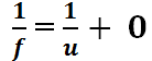
    similarly at the (1/u) intercept, the the value of (1/v) =0

    and so the lens formula becomes

    hence

    from the graph, we can deduce that 1/u and 1/v gives 1/f at the intercepts.

    we can get two values of f from the 1/v and 1/u intercepts such that:

    f1 = (1/v)-1 and f2 = (1/u)-1

    the focal length f is thus the average of f1 and f2 such that

    Related Topics


    References:
    • Secondary Physics Student’s Book Four. 3rd ed., Kenya Literature Bureau, 2012. pp. 1-42.
    • Abbot A. F. (1980), Ordinary Level Physics, 3rd Edition, Heinemann Books International,
      London.
    • Nelkon M. and Parker P., (1987), Advanced Level Physics, Heinemann Educational
      Publishers, London.
    • Tom D., and Heather K. Cambridge IGCSE Physics. 3rd ed., Hodder Education, 2018, https://doi.org/978 1 4441 76421. pp. 106-142.

    1. Magnetic Field patterns For a straight conductor

      Experiments have shown that magnetic fields created by a current moving through a straight conductor forms concentric circles around the conductor. See the illustrations in figure below.

      To investigate the magnetic field patterns due to a straight conductor, you may need to set up apparatus similar to the following diagram.

      A card with a small hole at the center is held horizontally so that a conductor in a complete circuit is held vertically through the hole such that the cardboard and the wire are perpendicular to each other.

      Iron fillings are sprinkled on the cardboard and then disturbed gently after the switch is closed. when the iron fillings are allowed to settle after disturbance, they settle around the current carrying conductor as in a pattern close to the illustrations shown shown.

      if we are to represent that on a diagram, it should be circles around the conductor as shown.

      This shows that iron fillings settles in concentric circles around the conductor becoming less significant ast the distance from the conductor increases from the center of the circle horizontally.

      Drawing magnetic patterns using a compass.

      All you need is to remove the iron fillings from the cardboard . Simply open the circuit and collect the iron fillings from the card and then leave the setup as before but with a compass on the cardboard as in figure below.

      After closing the switch, note the direction of the compass needle. Now put a dot at the end of the needle and move the compass to start at the end and then make a dot at the end of the needle. Move the compass so that it’s position begins at the dot and repeat the same procedure until you have circumnavigated the wire to make the pattern as shown.

      You can repeat the above procedure by selecting another radius from the conductor and trace the compass needle pattern to see it’s pattern of turning as it moves around the conductor.

      The compass needle are aligned in a circle pointing in the clockwise direction as in the setup described above in all radius selected to study the pattern.

      If the direction of current was reversed by changing the battery polarity, the circles would be plotted pointing anticlockwise direction.

      Magnetic fields produced by a straight current carrying conductor forms a pattern of concentric circles around the conductor.

      The direction of the magnetic field produced by a straight current carrying conductor can be predicted by use of Fleming’s-Right hand grip rule which states that:

      Use of Fleming’s Right-hand grip rule is illustrated below

      illustrating Fleming’s Right-hand grip rule

      Direction of the magnetic field around straight conductor can also be determined by use of Maxwell’s corkscrew rule which states that:

      The figure below illustrated Maxwell’s corkscrew rule:

      when using the Maxwell’s corkscrew rule, you imagine fastening the screw if the current is getting in to paper and you imagine removing the screw when current is moving out of the paper.

      Related Topics

      References

      • Secondary Physics Student’s Book Four. 3rd ed., Kenya Literature Bureau, 2012.
      • Tom D., and Heather K. Cambridge IGCSE Physics. 3rd ed., Hodder Education, 2018.

    2. Direction of induced current in a straight conductor

      Direction of induced current in a straight conductor

      consider the setup below

      To investigate direction of current on the straight conductor AB, you can do the following:

      • Move the condutor to cut the magnetic fields vertically upwards and note the direction of the magnetic field.
      • Move the condutor to cut the magnetic fields vertically downwards wards and note the direction of the magnetic field.
      • Hold the wire stationary in the magnetic field and note the deflection

      when the wire is moved upwards, the deflection on the galvanometer goes right showing that the current is flowing from A to B. To represent that on a paper, the induced current is envisioned to be moving into the page away from the eye as in the following illustration.

      when moved and when the wire is moved downwards deflections goes left showing that the current is moving from A to B . The current flow can be represented on a paper with current fl0wing out of the page towards the eye as in figure below.

      Fleming’s Right-hand rule

      Direction of an induced current in a straight conductor can be determined by Fleming’s right-hand rule which states that:

      The figure below shows how your right hand should be held to determine the direction of the induced current by use of Flemings’s right hand rule.

      Fleming’s right hand rule is also known as the dynamo rule and it agrees with the Lenz’s law.

      Consider a horizontal magnet held as shown in figure below:

      The direction of the magnetic field is downward. The downward direction of the above magnetic field can be represent by a section of an arrow tail to show that the magnetic field is going down into the paper.

      Suppose we have a conductor that is held horizontally between the two poles, the conductor will slide away or towards the magnet if it has some current flowing in it.

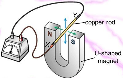
      The figure below shows current through a certain conductor XY inside a magnetic field moving into the paper and the likely motion for such a setup.

      According to Fleming’s rule which is consistent with the lenz’s law, the current must flow from X to Y in order to produce an electromotive force that is to push the rod XY to the right.

      Related topics


      References

      • Secondary Physics Student’s Book Four. 3rd ed., Kenya Literature Bureau, 2012.
      • Tom D., and Heather K. Cambridge IGCSE Physics. 3rd ed., Hodder Education, 2018.

    3. The Lenz’s law

      Consider the setup illustrated in the diagram below

      When the magnet is moved towards the coil, the galvanometer deflects and when moved away, the deflection happens in the opposite direction. This shows that the direction of change of the magnetic flux linkage determines direction of the induced current.

      Galvanometer deflection according to direction of current

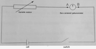
      We need to investigate how the current flows depending on the direction of the magnetic flux change and so we setup an experimental apparatus as shown.

      To investigate about current direction, we manipulate the apparatus in the following ways:

      • Adjust the variable resistor to a high value in order to limit the current through the sensitive galvanometer.
      • Close the switch and note the deflection on the galvanometer when current flows from A to B.

      When current direction is from enter galvanometer through A and leave at B, The deflection on the galvanometer is to the right. From the diagram, the current leaves the cell towards A.

      If the cell is reversed such that the current enters the galvanometer through B, the deflection happens to the left.

      Determining direction of the induced current

      Consider a coil of wire and a galvanometer connected as shown with a magnet being moved towards the coil.

      When the north pole of the magnet is moved towards the coil, the galvanometer deflects to the left indicating that the direction of the induced current is clockwise as in the direction DCBA.

      When the north pole of the magnet is moved away from the coil, the pointer deflects to the right indicating that current flow is in the anticlockwise direction or direction DABC.

      As the north pole of the magnet moves towards the coil, the induced current flows in the coil in an attempt to form an electromagnet with a north pole at the end near the incoming magnetic pole. This is meant to resist movement of the incoming north pole. From the clock rule studied in magnetic Effect of electric current, The current flow in the conductor will be as illustrated below so that the end near the north pole forms an opposing north pole.

      Remember the basic law of magnetism states that:

      When the North pole of the magnet is moved away from the coil, the induced current in the coil flows in such a way that a south pole is formed at the end of the coil near the leaving magnet so as to oppose movement of the receding magnet. Using the clock rule, the direction of induced current flow is as illustrated in the diagram below.

      From the above experiments and observations, the direction of the induced current in a coil can be determined in Lenz’s law which states that:

      Lenz’s law applies the principle the principle of conservation of energy. The mechanical energy used to move the magnet to the coil is converted to electrical energy in the form of an induced current. Work is done by the hard pushing the magnet towards the coil against the repulsive force from the induced pole of the coil if the current has to flow.

      Related topics


    4. Factors Affecting Magnitude of an Induced EMF

      Electromagnetic induction is one of the most important concepts in physics, describing how an electromotive force (EMF) is generated when the magnetic flux linking a conductor changes. This principle forms the basis of many electrical devices, including generators, transformers, and induction cookers. However, the magnitude of the induced EMF is not always the same; it depends on several factors that influence the rate at which magnetic flux changes. Understanding these factors helps explain how electrical energy is produced efficiently and why certain induction systems generate larger voltages than others. In this article, we explore the key factors that affect the magnitude of an induced EMF and their practical applications in modern technology.

      The amount of current produced from changing magnetic flux depends on a number of factors which includes:

      • Rate of change of magnetic flux
      • strength of magnetic field
      • number of turns in a coil
      i. Rate of change of magnetic flux

      The faster the rate of change of magnetic field, the higher the magnitude of the induced current.

      Consider a coil of about 200 turns of a wire, sensitive galvanometer and a magnet arranged as shown in figure below.

      To investigate how rate of change of magnetic flux, you move the magnet towards the coil and away at various speeds such as very fast, moderately fast and slowly.

      You observe that the faster the magnet is moved to and from the coil, the higher the deflection on the galvanometer. This shows that induced EMF is highest when the rate of change of magnetic flux is highest.

      Magnetic flux could be interpreted as the number of magnetic field touching the coil at any given moment.

      Magnetic flux Φ is the strength of magnetic field threading a given area.

      The magnetic flux Φ changes when the magnet is withdrawn from the coil where a faster withdrawal gives rise to a higher rate of change in magnetic flux linking the coil which then gives an increased induced Electromotive force(e.m.f)

      see the diagram below that shows magnetic field lines:

      ii. strength of magnetic field

      Moving a stronger magnetic towards or away from the coil causes increase of the induced current when the speed of movement remains constant.

      Consider a u-shaped electromagnet and a variable resistor connected to a circuit shown such that an electromagnet can have it’s strength varied by changing current passing through using the variable resistor.

      illustrating factors that affects induced emf

      After the setup, you can do the following to investigate the current induced with strength of the magnet:

      • Adjust the variable resistor so that minimum current flows.
      • Move the conductor PQ in a direction perpendicular to the magnetic field of the electromagnet and note deflection on the galvanometer.
      • change values of current and record corresponding readings on the galvanometer when wire cuts across the magnetic field.

      Whenever current through the ammeter is increased, a greater deflection is obtained on the galvanometer when the conductor wire cuts across the magnetic field.

      Higher current passing through a coil of wire leads to a stronger electromagnet that will produce stronger magnetic field .

      We can therefore conclude that the magnitude of the induced current is directly proportional to the strength of the magnetic field from which it is being produced.

      iii. number of turns in a coil

      If all other factors are held constant but the number of turns of wire on the coil increased, the induced current is observed to increase proportionately to increased number of turns.

      Having at your disposal insulated copper wire, sensitive galvanometer, magnet and connecting cables, you make a coil of numbered turns of wire and set up the apparatus as shown

      to investigate how number of turns in a coil affects magnitude of the induced emf, do the following:

      • Insert a magnet in the coil and then withdraw it at a steady speed and then observe and record the maximum reading on the galvanometer.
      • Increase number of turns on the coil at equal intervals says 50, 100,150,200,250 etc and repeat the above procedure noting the maximum deflection each time.

      Each time the number of turns of the coil is increased and all other factors held constant, a higher deflection on the galvanometer is recorded. The deflection is proportional to the number of turns used.

      Increased deflection indicates more current is produced in the coil. The induced emf is proportional to the number of turns and so we can say that each turn on the coil induces it’s own e.m.f. The total induced e.m.f is therefore a summation of all emfs produced by individual turns.

      Infact by application of calculus, we can be able to express summation mathematically, but we will do that later in more advanced lessons.

      Conclusions

      Experiments shows that an e.m.f is induced in a circuit whenever magnetic flux linkage changes and the magnitude of the induced e.m.f increases with increase in the rate of change of the flux linkage and the number of turns of the coil.

      The observations from experiments can be summarized in a Faraday’s law of electromagnetic induction which states that:

      practice exercise

      ⚡ Factors Affecting Magnitude of an Induced EMF – Revision Exercise

      Answer all questions and click Submit Quiz to see your score.

      1. Electromagnetic induction occurs when:

      2. The SI unit of induced electromotive force is:

      3. Which factor does NOT affect the magnitude of induced EMF according to the article?

      4. The faster a magnet is moved towards a coil:

      5. Magnetic flux can be interpreted as:

      6. A galvanometer is used to measure:

      7. If a magnet is withdrawn faster from a coil, the induced EMF:

      8. Increasing the strength of a magnetic field will:

      9. In the electromagnet experiment, magnetic field strength was changed using:

      10. A stronger electromagnet is produced by:

      11. Increasing the number of turns on a coil causes:

      12. The induced EMF is proportional to:

      13. Which instrument showed larger deflection when more EMF was induced?

      14. If all factors remain constant except the number of turns doubles, the induced EMF will:

      15. Magnetic flux Φ refers to:

      16. The greater the rate of change of magnetic flux linkage, the:

      17. Faraday’s law states that induced EMF is directly proportional to:

      18. Which device is based on electromagnetic induction?

      19. Increased galvanometer deflection indicates:

      20. Each turn of a coil contributes:


      Related topics


      References

      • Secondary Physics Student’s Book Four. 3rd ed., Kenya Literature Bureau, 2012.
      • Tom D., and Heather K. Cambridge IGCSE Physics. 3rd ed., Hodder Education, 2018, https://doi.org/978 1 4441 76421.

    5. Hans Ørsted

      Hans Christian Ørsted (1777-1851) was a Danish physicist and chemist who discovered that electric currents create magnetic fields, leading to the concept of electromagnetism. This discovery laid the foundation for the development of many technologies, including electrical power generation, motors, and telecommunications. Ørsted is considered one of the founding fathers of electromagnetism along with scientists like Michael Faraday and André-Marie Ampère.

      His Birth

      Hans Christian Ørsted was born in Rudkøbing, Denmark, on August 14, 1777.
      He was the child out of ten born by Mr. Søren Christian Ørsted and Mrs Karen Hermansen Ørsted. They lived in Rudkøbing, Denmark, where Hans Christian Ørsted was born.

      His father, Søren Christian Ørsted, was a pharmacist by profession. His mother, Karen Hermansen Ørsted, was the daughter of a merchant. While Søren Christian Ørsted worked as a pharmacist, he also had interests in natural philosophy, which may have influenced Hans Christian Ørsted’s later pursuits in science.

      Siblings

      Mr. Søren Christian Ørsted children in the order of birth is as follow:

      1. Anders Sandøe Ørsted (1778–1860)
      2. Hans Christian Ørsted (1777–1851)
      3. Jacob Ørsted (1782–1819)
      4. Christian Ørsted (1783–1843)
      5. Joachim Ørsted (1785–1854)
      6. Hans Peter Ørsted (1788–1842)
      7. Anton Ørsted (1791–1860)
      8. Anna Ørsted (1792–1837)
      9. Johan Rudolph Ørsted (1794–1866)
      10. Karen Margrethe Ørsted (1797–1884)

      Early life

      From a young age, he showed an interest in science and natural philosophy. He was fortunate to have access to a good education, attending school in Copenhagen and later studying at the University of Copenhagen.

      Ørsted initially pursued a degree in medicine, as was common for students of natural philosophy at the time, but his interests soon shifted towards physics and chemistry. He was greatly influenced by the works of scientists like Isaac Newton and Johann Wilhelm Ritter.

      After completing his education, Ørsted embarked on a journey of scientific exploration and discovery. He conducted experiments in various fields of physics and chemistry, including acoustics, optics, and electricity. His most famous discovery came in 1820 when he observed that electric currents could create magnetic fields, leading to the development of the concept of electromagnetism.

      Throughout his life, Ørsted was deeply engaged in scientific research and education. He held various academic positions, including professorships at the University of Copenhagen, where he inspired numerous students with his passion for science. Ørsted’s contributions to the field of electromagnetism laid the foundation for modern physics and earned him international acclaim.

      Beyond his scientific achievements, Ørsted was also involved in cultural and philosophical pursuits. He wrote extensively on topics ranging from aesthetics to the unity of the physical sciences.

      Overall, the early life of Hans Christian Ørsted was characterized by intellectual curiosity, a thirst for knowledge, and a relentless pursuit of scientific truth. His groundbreaking discoveries continue to influence scientific research to this day.

      Schooling

      Hans Christian Ørsted attended various schools during his early education. He began his schooling in Rudkøbing, Denmark, where he was born. Later, he attended the Cathedral School in Horsens, Denmark. After completing his primary education, Ørsted continued his studies at the University of Copenhagen, where he pursued a degree in medicine. While at the university, he became increasingly interested in physics and natural philosophy, eventually leading him to make significant contributions to the field of electromagnetism.

      Oersted Marriage

      Hans Christian Ørsted married twice in his lifetime.

      His first marriage was to Inger Birgitte Ballum on June 1, 1814. They had six children together: two sons, Christian and Carl, and four daughters, Mathilde, Henriette, Charlotte, and Harriet. Sadly, his first wife, Inger, passed away in 1829.

      In 1831, Ørsted married his second wife, Magdalene Cathrine Hanck. Their marriage lasted until Ørsted’s death in 1851. He did not have any children with his second wife

      His children

      Hans Christian Ørsted had six children with his first wife, Inger Birgitte Ballum. These children were born between the years of 1815 and 1828. Their names, in order of birth, were:

      1. Christian Ørsted
      2. Carl Ørsted
      3. Mathilde Ørsted
      4. Henriette Ørsted
      5. Charlotte Ørsted
      6. Harriet Ørsted

      There isn’t extensive information readily available about the specific career paths or achievements of Hans Christian Ørsted’s children. However, it’s worth noting that Christian Ørsted, his eldest son, followed in his father’s footsteps to some extent. Christian became a botanist and made contributions to the study of algae

      Achievements

      Here are some of Hans Christian Ørsted’s key achievements:

      Ørsted discovered the phenomenon of electromagnetism on April 21, 1820, while conducting an experiment at the University of Copenhagen. This discovery demonstrated the relationship between electric currents and magnetic fields.

      Ørsted published his findings on electromagnetism in a paper titled “Experiments on the Effect of a Current of Electricity on the Magnetic Needle” in July 1820. This publication provided a detailed account of his experiments and observations.

      On September 16, 1820, Ørsted demonstrated that an electric current could produce mechanical motion by causing a wire carrying the current to rotate around a magnetic needle. This experiment further confirmed the connection between electricity and magnetism.

      Following his initial discovery, Ørsted continued to investigate the relationship between electric currents and magnetic fields. His work contributed to the development of electromagnetic theory, which was further advanced by scientists like André-Marie Ampère and Michael Faraday.

      In addition to his work in electromagnetism, Ørsted made significant contributions to chemistry throughout his career. He conducted research on the properties of gases and the nature of chemical bonds, contributing to advancements in chemical theory.

      Ørsted was known for his meticulous experimental approach to scientific research. He conducted numerous experiments in various fields, including acoustics, optics, and thermodynamics. His commitment to empirical investigation helped to advance scientific knowledge and understanding.

      Ørsted was deeply involved in academia throughout his life. He held various academic positions, including professorships at the University of Copenhagen, where he inspired and mentored numerous students. He also played a key role in reforming science education in Denmark, advocating for a more practical and experimental approach to learning.

      Oersted’s death

      Hans Christian Ørsted died on March 9, 1851 following a stroke. He passed away in Copenhagen, Denmark, at the age of 73. Ørsted’s death marked the end of a remarkable career filled with scientific achievements and contributions to the fields of physics, chemistry, and education.

      His political ideologies


      Hans Christian Ørsted was known for his engagement in politics, particularly during a time of political change in Denmark. He was associated with the Danish Golden Age, a period of cultural flourishing in Denmark during the early 19th century.

      Ørsted held liberal political views and was actively involved in political discussions and movements of his time. He advocated for constitutional reforms and supported the idea of a constitutional monarchy. He also participated in debates on education and civil liberties, emphasizing the importance of scientific education and freedom of thought.

      Ørsted’s political affiliations aligned with the broader cultural and intellectual currents of the Danish Golden Age, which emphasized enlightenment ideals, liberalism, and cultural nationalism. However, it’s important to note that his primary legacy remains his scientific achievements rather than his political activities.

      Religious inclinations

      Hans Christian Ørsted was raised in a Lutheran household, as Denmark, his home country, is historically predominantly Lutheran. While there isn’t extensive documentation regarding his personal religious beliefs or practices, it’s generally assumed that he identified with the Lutheran Church, which was the state religion of Denmark at the time.

      However, Ørsted was also known for his philosophical and intellectual pursuits, which included reflections on the relationship between science and spirituality. He was influenced by Romantic and idealistic philosophies, which sometimes explored spiritual themes alongside scientific inquiry.

      Overall, while Ørsted’s religious inclinations likely reflected the cultural context of his upbringing, his primary focus and legacy were in the realm of science and scientific discovery.

      Close associates

      Hans Christian Ørsted had several close associates and collaborators throughout his life, particularly in the scientific and academic communities. Some of his notable associates include:

      i. Anders Sandøe Ørsted

      Anders Sandøe Ørsted was Hans Christian Ørsted’s older brother. While not as famous as his brother, Anders was a lawyer, politician, and writer. The brothers had a close relationship, and Anders provided support and encouragement for Hans Christian’s scientific pursuits.

      ii. Johan Ludvig Heiberg

      Johan Ludvig Heiberg was a Danish mathematician, physicist, and philosopher who collaborated with Ørsted on various scientific endeavors. Heiberg was a prominent figure in the Danish academic community during the early 19th century.

      iii. Johan Nicolai Madvig

      Johan Nicolai Madvig was a Danish philologist and politician who worked closely with Ørsted in educational and political reforms in Denmark. Madvig was a strong advocate for educational improvements and served in various official capacities in Denmark.

      iv. H.C. Ørsted Institute

      The H.C. Ørsted Institute, named in honor of Hans Christian Ørsted, is a research institute at the University of Copenhagen. It was established in 1920 to promote research and education in the natural sciences, continuing Ørsted’s legacy in scientific inquiry.

      v. Students and Colleagues

      Throughout his career as a professor at the University of Copenhagen, Ørsted mentored numerous students and collaborated with colleagues in scientific research and academic endeavors. His influence extended beyond Denmark, as his discoveries in electromagnetism had a profound impact on the development of physics worldwide.

      These individuals and institutions played important roles in Ørsted’s life and career, supporting his scientific endeavors, advocating for educational reforms, and contributing to the broader intellectual and cultural landscape of Denmark during

      Related Topics


    6. Vector Addition

      Addition of two vectors may be affected with the help of parallelogram law of addition.

      The resultant(sum) vector R’ of A’ and B’ is the diagonal of the parallelogram of A and B of adjacent sides.

      The triangular law of vector addition follows the parallelogram law which states that: if the tail-end of the vector is placed at the arrow-head of the vector, their resultant(sum) vector is drawn from the tail of the first to the head of the other.

      see the figure below

      Subtraction of vectors

      The figure below shows addition of vectors in reverse direction of B’ vector.

      The process of subtracting one algebraic quantity from one another is equivalent to adding the negative of the quantity to be subtracted. in essence, a-b = a+(-b)

      The negative vector –B‘ of vector B is defined as a vector of the same magnitude(length) but in opposite direction.

      Resultant set of forces

      Two vectors are said to be equal if they have the same magnitude and direction. If two vectors A and B are parallel, the magnitude of vector sum C equals the sum of magnitudes of A and B.

      consider the vectors A and B represented below

      The resultant vector C will be represented by a single vector as shown

      If two vectors are antiparallel, the magnitude of a vector equals the difference of the magnitudes of A and B

      The diagram below shows vectors that represents forces acting in opposite direction

      The resultant vector is smaller than the larger vector and bigger than the smaller vector and moves in the direction of the larger vector.

      Related Topics


      References
    7. Conical Pendulum

      Conical Pendulum

      The diagram below represents a body of mass m moving on a horizontal circle with a constant velocity v at the edge of a cord of length L.

      As the body swings around it’s path the cord swings over the surface of a cord. The cord makes an angle θ with the vertical so that the radius of the circle in which the moves is R=Lsinθ and the magnitude of the velocity is given by:

      where T is the periodic time.(time for one complete revolution).

      The forces exerted on the body when it is in the position shown are it’s weight(mg) and tension(T) in the cord.

      Tension T can be resolved into horizontal and vertical component Tsinθ and Tcosθ respectively.The body has no vertical acceleration, so the vertical forces Tcosθ and mg are equal in magnitude.

      The resultant inward radial(centripetal) force is the horizontal component Tsinθ which is equal to the mass(m) multiplied by the radial or centripetal acceleration.

      From linear motion, F=ma.

      but since the motion is circular; a=v2/r

      hence, the expression for the horizontal motion.

      For the vertical forces;

      Tsinθ = mg ……………………………….. (ii)

      When the equation (i) is divided by equation (ii) the result is:

      but from trigonometry, sinθ/cosθ = tanθ; hence

      When we make use of the relation r = L sinθ and v = 2πLsinθ/T

      The equation becomes:

      This leads to:

      hence we have;

      dividing by sinθ on both sides;

      from the equation tanθ = sinθ/cosθ ; 1/cosθ = tanθ/sinθ and therefore:

      and hence;

      and making T the subject of the formular, we have;

      which will results to:

      The angle θ depends on the time of revolution T and the length of the cord.

      For a given length L, cosθ decreases as the time is made shorter and shorter and the angle θ increases. The angle θ never becomes 90o sinces this requires that T = 0 or v= .

      The largest possible value of T is given by T=2π√l/g which occurs for a very small angle θ for which cosθ=1 and therefore:

      Related topics

      References

      • Sanny, J. S., & Ling, S. (2016). University Physics Volume 1. OpenStax. https://doi.org/13: 9781938168161
      • Abbott, A. F. (1989). PHYSICS (5th ed.). Heinemann. https://doi.org/978043567014
    8. Equilibrium and center of gravity

      Equilibrium and center of gravity

      An object is considered to be made up very many particles that are joined together to form the whole object.

      Each particle in an object experiences gravitational attraction.

      The figure below illustrates particles of solid experiencing gravitational attraction. Each particle will have weight w assuming that all the particles are of same mass.

      Gravitational attraction is the force between two bodies of given mass.

      Any object or particle that has some mass will be attracted towards the centre of the earth. The force of attraction on any particle or object of mass m by Earth’s attraction on it is given as w=mg.

      This force on an object by the earth’s gravitational force is the weight of the object.

      The weight of all the particles in the object sums up to provide the weight of the object. The sum of these gravitational attractions on all particles of an object acts through one point in an object called centre of gravity.

      The figure below illustrates a straight metal rod with tiny particles experiencing some gravitational pull.

      if moments were taken about point o, such that the sum of moments about it from the left or right of o balances, then the straight rod will balance at o without toppling. Point o is then said to be the centre of gravity of the metal rod.

      The centre of gravity of a body is defined as the point of application of the resultant force due to earth’s attraction on the body.

      some books defines center of gravity as a point on a body or system where force of gravity can be considered to act. It is the point in any object about which the object is in perfect balance no matter how it is turned or rotated around that point.

      Most often, the center of gravity of bodies with a regular shape is also the geometrical center of that body. The mass of such a body is said to be uniformly distributed. For Example when we cut a straight metal rod illustrated earlier into pieces of equal length, then each piece cut will be having equal mass and consequently, the mass of the straight rod is proportional to it’s length.

      The center of gravity of an irregular object is closer to the part that has more particles or where most of the mass is concentrated.

      Center of gravity and the state of balance

      A support placed at a point on the centre of gravity of an object places the object in a state of balance so that it does not turn or tip. This is because the weight of an object acts through the center of gravity of an object.

      If a pivot is some distance from the center of gravity of an object, the object tips off in the direction of the weight, this is because the weight of an object causes the turning effect to a pivoted object.

      Example

      A uniform metal bar 160 cm long is pivoted at 30 cm mark such that it balances when a mass of 2.0 kg is attached at 0 cm mark as shown in figure 4.5. Calculate the weight of the bar.(take g=10Nkg-1)

      solution

      This metal bar is a uniform body and so it’s mass is evenly distributed, therefore it’s weight will act at its geometrical center. The weight will act at the 80 cm mark as shown because it is the center of the bar as shown.

      The moments due to weight balances with moments due to the mass at the 0 cm mark on the metal road.

      the distance from weight to the pivot =50 cm = 0.5 m

      distance from 2.0kg mass from the pivot is 30 cm = 0.3 m.

      the weight of the mass is 2.0kg x 10Nkg-1 = 20.0N

      The clockwise moments will be given by W x 0.5 m

      Anticlockwise moments will be given by 20.0 N x 0.30 m

      from the principles of moments:

      20.0 N x 0.30 m = W x 0.5 m

      equation to calculate weight of the object
      Exercise Problems

      An object is pivoted such that it is balanced by a force of 4.0 N placed 70 cm from the fulcrum. If the weight of the object acts at 55 cm from the fulcrum on the opposite side,find the center of gravity of the object and it’s mass.

      Answers:

      • center of gravity is 125 cm from one end
      • the mass is approximately 5.091 kg
      Related topics

    9. Heat conduction

      Heat conduction

      Heat conduction is a process by which heat moves in solids by means of vibrations of it’s molecules.

      If you put one end of iron on fire, soon it the other end will be hot, sometimes too hot to handle. The heat energy entering the iron from the hot end increases the vibrations of atoms in that end which then collides with their neighbouring atoms, increasing vibrations of the neighbour atoms and hence passing the heat energy along.

      Metals have free electrons which travels throughout the body freely and randomly. Heat energy injected at the hot end of a metal increases vibrations of the particles at that end causing the free electrons in that region to gain more kinetic energy and because they are moving freely, they carry energy to other parts of the metal making heat conduction in metal faster than in other forms of matter.

      Different solids conducts heat differently, where some solids like aluminium conducts heats very fast whereas rate of heat transfer in wood and rubber is extremely slow, almost zero.

      to compare heat conduction of various materials, consider an experiment with the following materials:

      • Rods of aluminium
      • iron
      • rubber
      • glass
      • wood
      • source of heat
      • thermal conductivity tank

      The materials listed should be of the same length and thickness.

      procedure

      • setup the apparatus as shown ensuring that the rods are firmly held before poring boiling water into the water bath.
      • observe the order in which was of solid fat fixed at the end of the materials will melt and fall from the rod it is fixed.
      observations

      The wax on end of copper rod melts before any other, then it was followed with the one on aluminium and the one on iron was third.

      This shows that copper conducts heat faster compared to aluminium and aluminium conducts heat faster compared to iron.

      wax on glass will melt after sometimes but the one on wood and rubber will not melt. In fact the boiling water will cold before they melt.

      Explanations

      Different materials have different thermal conductivity with metals being generally good conductors of heat and non metals being poor conductors of heat.

      solids that are poor conductors of heat only conducts heat by vibrations of atoms which can be slow and don’t have free electrons to move heat faster.

      poor conductors of heat are very useful because they are usually used as insulators where we need to prevent heat flow.

      Good conductors of heat are also very useful in making of cooking pots and heat sinks.

      Sometimes we need good conductors of heat and other times we need poor conductors when heat movement is not desirable. So both poor and good conductors are important to us. None is more important than the other.

      some of the good conductors of heat in decreasing rate of conduction includes:

      • silver
      • copper
      • aluminium
      • brass
      • zinc
      • iron
      • lead
      • mercury

      some of the poor conductors of heat in decreasing rate of conduction includes:

      • concrete
      • glass
      • brick
      • asbestos paper
      • rubber
      • wood
      • water
      • air

      Related topics